In this project Tweets featuring the word "conservation" and a sample of messages from zoochat.com, a conservation message board, will be text mined and analysed.
Analysis will determine what the most prevalent conservation topics are being spoken about online.
More specifically the following questions will be answered:
What geographical locations or habitat types are most talked about online in regard to biological conservation?
What animal taxa receive the most conservation effort and/or public attention?
What public institutions are most associated with conservation?
The first step is to mine the HTML files from zoochat.com.
# Call the 'Rcrawler' package
library(Rcrawler)
# Add the website URL and specify the download location
Rcrawler(Website = "https://www.zoochat.com/community/",
DIR = "C:\\Users\\james\\Documents\\Crawled Pages")
For this project 1% of the zoochat site was crawled and downloaded.
The next step is to crawl Twitter. Downloading Tweets requires permission from the Twitter which can be gained by applying for a developer's site account.
Once applied and logged in, four passwords can be produced on the site. These must be included when producing a token to signify that permission has been obtained.
# Create the permission token using the four passwords (left blank here)
# Create a unique function using a function from the 'tm' package where 'x' is the corpus name and 'pattern' is the pattern of text to be removed from the character string
Now the text in the corpus is clean the next step is to coerce and store the corpus as a Document Term Matrix so the text terms can then be listed, ordered and analysed.
# Store the corpus as a DTM while setting a minimum and maximum word length to exclude anything missed by the clean up
# Also set a minimum of term frequencies to be included in the DTM - terms occuring 3 times or less will be excluded
dtmconserv <- DocumentTermMatrix(conservdocs,
control = list(wordLengths=c(4,20),
bounds=list(global=c(3, 27))))
# Create a list using the DTM where one column will have terms and another will have the frequency of terms
freqconserv <- colSums(as.matrix(dtmconserv))
# Create an index for the list indicating that the most frequent terms should appear first
ordconserv <- order(freqconserv, decreasing = T)
# Apply the index
freqconserv <- freqconserv[ordconserv]
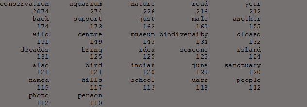
# Call a sample of the list
freqconserv[1:32]
This shows a small sample of the list. Text Mining and analysis is an interative process and will usually involve manual removal of unwanted terms.
For example the sample list shows the stop word "also" and part of a HTML command "uarr", have slipped through.
# Coerce the list as a matrix
freqconserv <- as.matrix(freqconserv)
# Locate the unwanted term's place in the list and remove
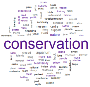
Here, a word cloud represents the most frequent words as larger and less frequent as smaller. Unsurprisingly "conservation" occurs the most as well as well-known locations.
Animal taxa names and other terms related to this subject, such as "biodiversity", are also shown to occur frequently.
An unfamiliar term that occurred frequently was "vogelcommando", a quick internet search revealed this is a user-name that posts frequently on the zoochat website.
Histograms can be created to visualise the frequency of terms related to the specific research questions.
# Create a data frame with the taxa terms and corresponding frequencies
plot1 <- ggplot(taxaterms, aes(Term, Occurences))
plot1 <- plot1 + geom_bar(stat="identity", fill = "purple4") +ggtitle("Frequency of Taxa Terms")
plot1
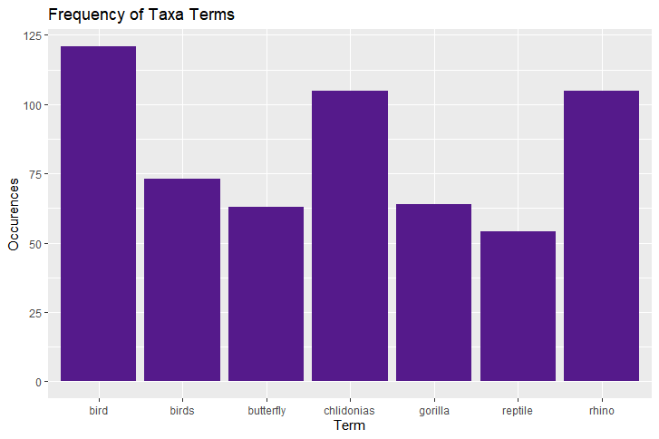
This reveals what animal taxa are being spoken about most recently in the context of conservation. This can either suggest which taxa are more popular among people or have received the most conservation effort recently.
The term "bird", "birds" and "chlidonias" (a genus of bird) occur very frequently. The specific use of taxa name "chlidonias" suggests that this taxa has been discussed in scientific context alot recently.
General taxa names such as "butterfly", "gorilla" and "reptile" suggest these taxa have been popular among the public and conservationists recently.
"Rhino" has also occurred frequently and is likely due to the recent International Rhino Day on 22/09/2020 (sites were crawled 24/09/2020).
# Create a data frame with the location terms and corresponding frequencies
plot2 <- ggplot(geolocterms, aes(Terms, Occurences))
plot2 <- plot2 + geom_bar(stat="identity", fill = "purple4") +ggtitle("Frequency of Geographical Location Terms")
plot2
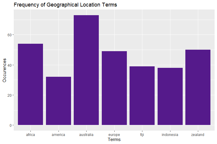
This histogram shows the frequency of country and continent terms (it should be noted for more detailed analyses cities, provinces and states would be included too). The minimum frequency threshold was lowered from 50 to 30 for this analysis as only two locations originally qualified.
The popularity of these locations is unsurprising due to the biodiversity in these tropical locations (assuming the term "america" is also referring to south America) and the first world (or 'well developed' where Fiji is concerned) status of these locations.
The term "australia" occurs much more frequently than the others, this is likely due to both aforementioned factors and responses to the damage caused by the 2019 bush fires.
# Create a data frame with the location terms and corresponding frequencies
plot3 <- ggplot(envirolocterms, aes(Terms, Occurences))
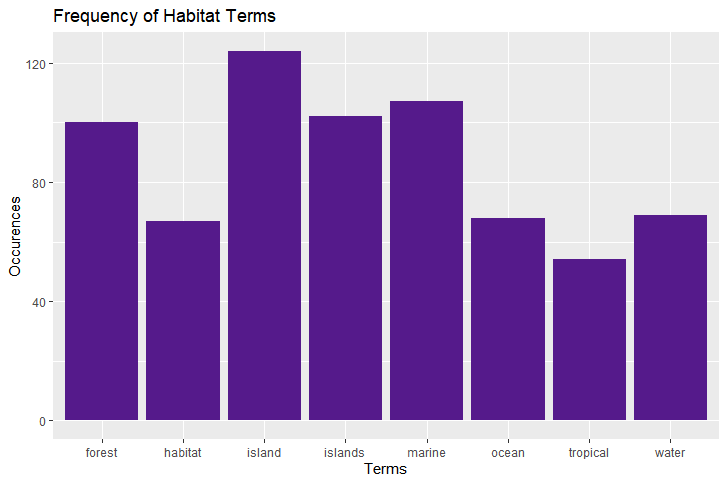
plot3 <- plot3 + geom_bar(stat="identity", fill = "purple4") +ggtitle("Frequency of Habitat Terms")
plot3
The high frequency of marine words ("island", "islands", "marine", "ocean", "water") suggests that people are highly concerned
with marine conservation.
This finding coupled with the fact no sea animal terms occurred more frequently than 50 times (refer to the taxa histogram)suggests that people are more concerned with saving the ocean in general rather saving specific marine species.
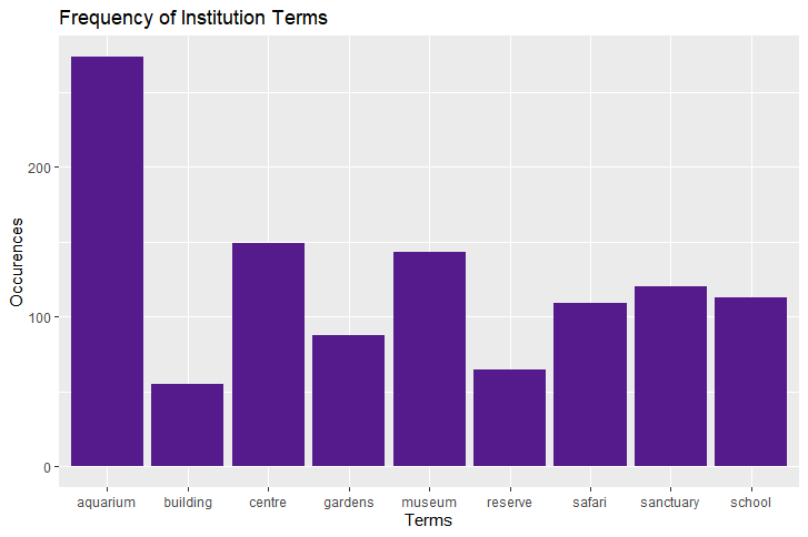
# Create a data frame with the institution terms and corresponding frequencies
plot4 <- ggplot(institterms, aes(Terms, Occurences))
plot4 <- plot5 + geom_bar(stat = "identity", fill = "purple4") +ggtitle("Frequency of Institution Terms")
plot4
This shows the number of times a conservation related institution was mentioned.
The term "aquarium" appeared much more frequently than any other institution term. This suggests that people in general are aware of the association between aquariums and marine conservation. Furthermore, this could show people are highly concerned with marine conservation.
An interesting finding is the lack of the term "zoo". This could be due to the tendency for twitter users to only use the word "zoo" in a hashtag (e.g "#ChesterZoo), the lack of spacing in this example would mean the text mining method will not identify "zoo" as an individual term. This is a drawback of the text mining method.
Another possibility is due to the public's perceptions of zoos. Zoos tend to be seen by the general public as a place for commercial entertainment and/or a "prison for animals". It is not common knowledge that zoos are a hub for conservation activities such as rescue, breeding and research. This could be the reason for the low frequency of this term.
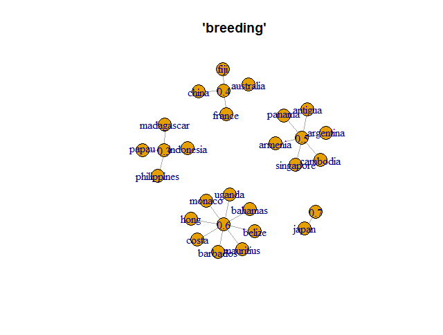
A Text Mining function can be used to determine the correlation between words, in this context this is the likelihood of one term appearing in the same document as another word.
This can be used to answer many interesting questions and will be used here to discover which countries are most strongly associated with captive breeding programmes online.
# Return a list of words associated with "breeding" with correlations stronger than 0.3
findAssocs(dtmconserv, "breeding", 0.3)
# Manually indentify the country terms and correlation values then create objects containing this information
This shows the correlations between country terms and the term "breeding" and could suggest which countries are most strongly associated with breeding programmes
However, there are drawbacks of answering questions using this method. In this instance "breeding" wasn't always referring to breeding programmes but were sometimes referring to the breeding of monkeys for testing in Mauritius or commercial swine breeding in the Bahamas.