The Flights dataset contains information on US domestic flights such as departure times/locations, arrival times/locations, airports used etc.
However, the original dataset is messy. The first aim of this project is to clean the dataset ready for analysis. The next aim is to perform a Logistic Regression in order to determine the odds of flight cancellations in regard to the departure US state.
# Import the txt file containing the dataset specifying the delimeters as "|"
The next step in the data clean up is the DISTANCE variable which shows the scheduled flight duration, however, it cannot be used in calculations in its current form due to its combination of numbers and characters.
head(flights$DISTANCE)
# Replace the string "miles" with absence of characters ("")
Say time of day needed to be used as a predictor variable (e.g. whether flights leaving in the AM or PM have an effect on a response variable) then we would need to use the departure times to create a new AM/PM variable.
# Check the departure times variables
head(flights$DEPTIME)
# Coerce the variable from a factor to a numeric vector
flights$DEPTIME <- as.numeric(flights$DEPTIME)
# Create the new variable name followed the requirements for the new value
# In this instance the requirements are whether times are before or after noon (i.e. 1200) they are then coded as AM or PM respectively in the new column
Now all rows will have an AM or PM value in a new column depending on their departure time.
That's it for miscellaneous data clean up.
Now its time to start the Logistic Regression.
The research in question is whether flights are more or less likely to be cancelled based on their departure state. So the CANCELLED variable will need to be prepared.
# Check the CANCELLED variable
unique(flights$CANCELLED)
Logistic Regression is used when the response variable has binomial data (1/0, Yes/No, Success/Failure). Therefore, the response variable CANCELLED must have values of either 1 or 0, where 1 represents a cancellation and 0 a non-cancellation.
# Must coerce the variable into a character string so "T" and "F" are recognised as letters rather than TRUE/FALSE logical values in R
# Use the index to create an 80% sized training dataset
train.flights <- flights[train.index,]
# Use the index to create a 20% sized testing dataset
test.flights <- flights[-train.index,]
# Fit a Logistic Regression model using the training dataset
train.model <- glm(CANCELLED ~
ORIGINSTATENAME,
data = train.flights,
family = "binomial")
# Call the summary statistics of the training model
summary(train.model)
Summary of the training model statistics show a few significant p-values (p < 0.05) which suggests there is a significant difference between the likelihood of cancellations when flights depart from different states.
The AIC value represents the level of prediction errors, where a higher AIC indicates the model is more likely to make preidction errors.
As a general rule, a model of less than 2000 is desirable, therefore the AIC value shown here suggests the final model (which will use 100% of the data) could be ineffective.
However, AIC values are primarily used for comparing different models. Because only one model is being fitted during this project, further diagnostics can be done to determine its effectiveness.
# This command will predict values using parameters from the training model
# This next command will indicate the accuracy of the model predictions by returning the mean of a set of values predicted by the training model while using true values from the CANCELLED variable as an index
# Using this index means only the mean prediction for the true outcomes are calculated
According to calculation the probability of the model correctly predicting a cancellation is 0.03% and correctly prediciting a non-cancellation is 0.02.
Although this suggests the final model would definitely be ineffective, further diagnostics can still be performed to test it.
A Receiver Operator Characteristic (ROC) curve plots the True Positive Rate against the False Positive Rate and can be used in the diagnosis of a Logistic Regression model.
# Load the ROCR package
library(ROCR)
# Create the curve using the predicted values and true values
# Create the graph specifying the True Positve Rate ("tpr") and False Positive Rate ("fpr") as axes
ROCRgraph <- performance(ROCRcurve, "tpr", "fpr")
plot(ROCRgraph, colorize = T)
When a plotted ROC crurve leans toward the true positive rate rather then false positive rate (i.e. there is more graph space underneath the curve) this would indicate the model is more likely to make true predictions.
Unfortunately, in this case the ROC curve suggests the the model is more likely to make false predictions.
A threshold value can be obtained from the ROC curve's threshold spectrum to create a Confusion Matrix. A Confusion Matrix compares true and false values predicted by the training model and can have different threshold levels applied to it based on whether discovering true positives or true negatives are more important to the research question.
In logistic Regression a low threshold is used when predicting true positive values is more important. Since the research question is regarding the occurence of flight cancellations, a low threshold will be used.
According to this curve's threhsold spectrum, located on the right side of the plot, a threshold ranging 0.02-0.08 should be used.
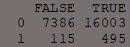
# Create a confusion using a low threshold value of 0.02 taken from the ROC curve
CM <- table(train.flights$CANCELLED,
predict.flights > 0.02)
CM
Results from the confusion matrix can be used to calculate the rate of accuracy.
The result from the Accuracy formula indicate that with a low threshold the model is somewhat accurate at approximately 69%.
Since this model uses categorical predictor variables, the best way to visualise results is by calculating and plotting the proportions of flight calculations departing from each state in the data set.
# Store the proportion of flight cancellations from each state
ggplot(cancellation.proportions, aes(x = State, y = Proportion))+
geom_bar(stat = "identity", color = "black", fill = "4")
It can be seen here that some states have a much higher proportion of cancellations than other states.
The next step is to fit the final model.
# Fit the final model using the full dataset
flights.model <- glm(flights$CANCELLED ~
flights$ORIGINSTATENAME,
data = flights,
family = "binomial")
# See the summary statistics
summary(flights.model)
From the model diagnosistics it is shown that this may not be the best model to use
to make predictions. However, with a very low threshold suggested by the ROC curve, the accuracy of the model calculated using values from a Confusion Matrix, is shown to be somewhat high.
Furthermore, p-values from the final model's summary statistics show that some flight origin states were signficantly more likely to have cancellations.
.png)
_2.png)
.png)
.png)
.png)
.png)
.png)
.png)

.png)
.png)